- Sequence processing
- Prepare environment
- Quality profiles of raw reads
- Filter raw reads
- Quality profiles of filtered reads
- Assess and plot errors
- Dereplicate
- Sample inference
- Generate sequence table
- Track reads through the pipeline
- Assign taxonomy
- Data preparation
- Ordering and colors
- Load the data
- Prepare tables
- Create phyloseq object
- Rarefaction
- Statistics & Visualization
- General overview
- Alpha diversity
- Venn diagrams
- Heatmap
- Ordination
- Permanova
- Pairwise Permanova
- LefSe
- Network
Bacteria
Sequence processing
Prepare environment
Load packages
library(tidyverse); packageVersion('tidyverse')
library(reshape2); packageVersion('reshape2')
library(ampvis2); packageVersion('ampvis2')
library(phyloseq); packageVersion('phyloseq')
library(microbiomeMarker); packageVersion('microbiomeMarker')
library(microbiome); packageVersion('microbiome')
library(RColorBrewer); packageVersion('RColorBrewer')
library(vegan); packageVersion('vegan')
library(ggpubr); packageVersion('ggpubr')
library(MicEco); packageVersion('MicEco')
library(RVAideMemoire); packageVersion('RVAideMemoire')
Set path and gather samples
path <- "...set path to your read files..."
list.files(path)

fnFs <- sort(list.files(path, pattern="_R1_001_trimmed.fastq", full.names = TRUE))
fnRs <- sort(list.files(path, pattern="_R2_001_trimmed.fastq", full.names = TRUE))

sample.names <- sapply(strsplit(basename(fnFs), "_"), `[`, 1)
Quality profiles of raw reads
plotQualityProfile(fnFs[1:2])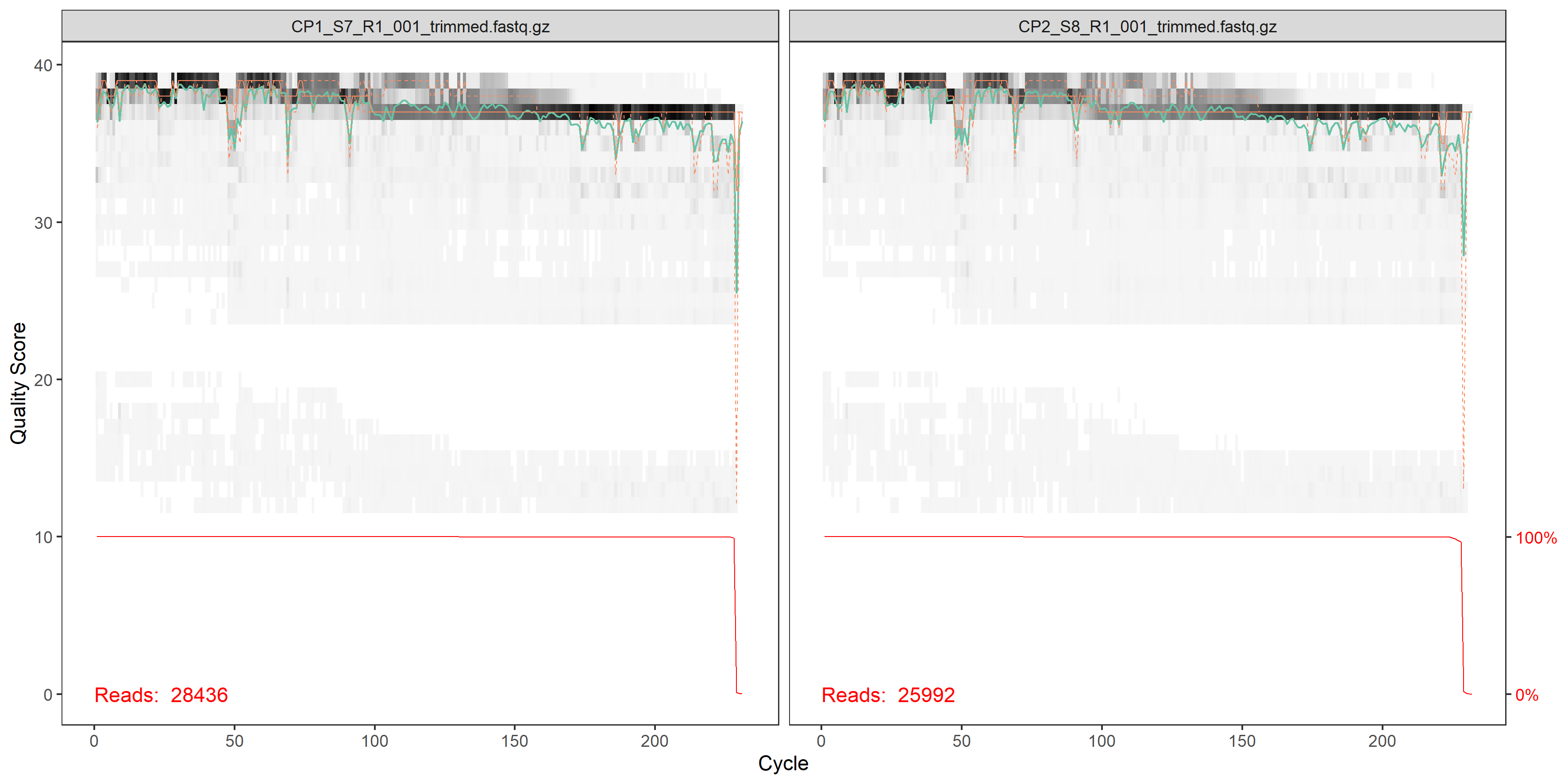
plotQualityProfile(fnRs[1:2])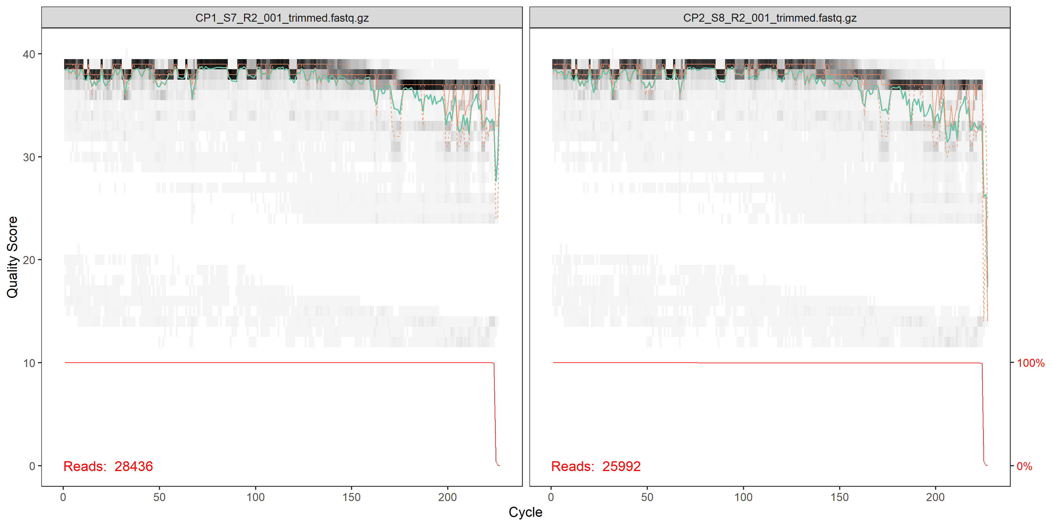
Filter raw reads
filtFs <- file.path(path, "filtered", paste0(sample.names, "_F_filt.fastq.gz"))
filtRs <- file.path(path, "filtered", paste0(sample.names, "_R_filt.fastq.gz"))

out <- filterAndTrim(fnFs, filtFs, fnRs, filtRs, truncLen=c(225,220),
                     maxN=0, maxEE=c(2,2), truncQ=2, rm.phix=TRUE,
                     compress=TRUE, multithread=FALSE)

outQuality profiles of filtered reads
plotQualityProfile(filtFs[1:2])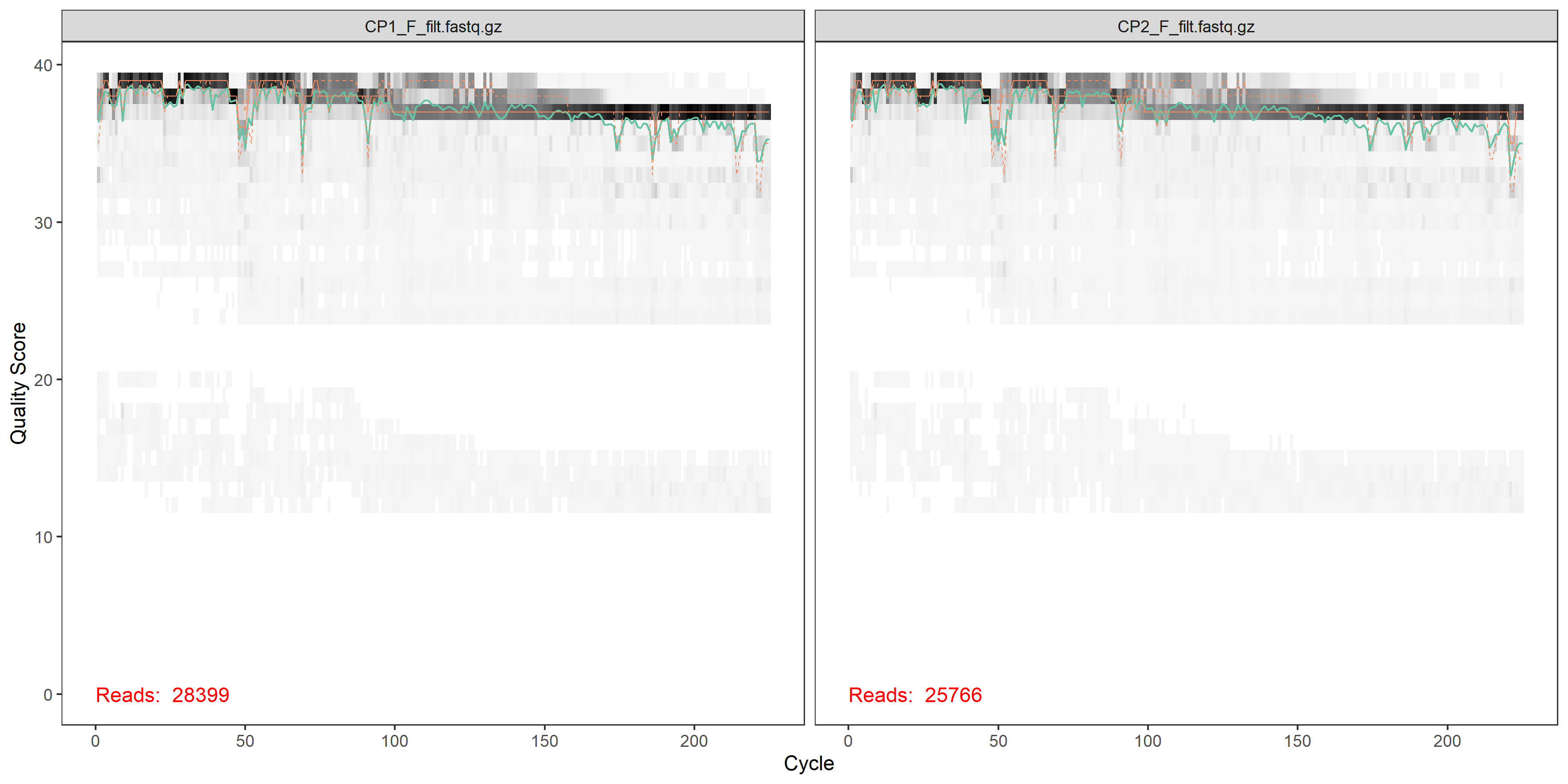
plotQualityProfile(filtRs[1:2])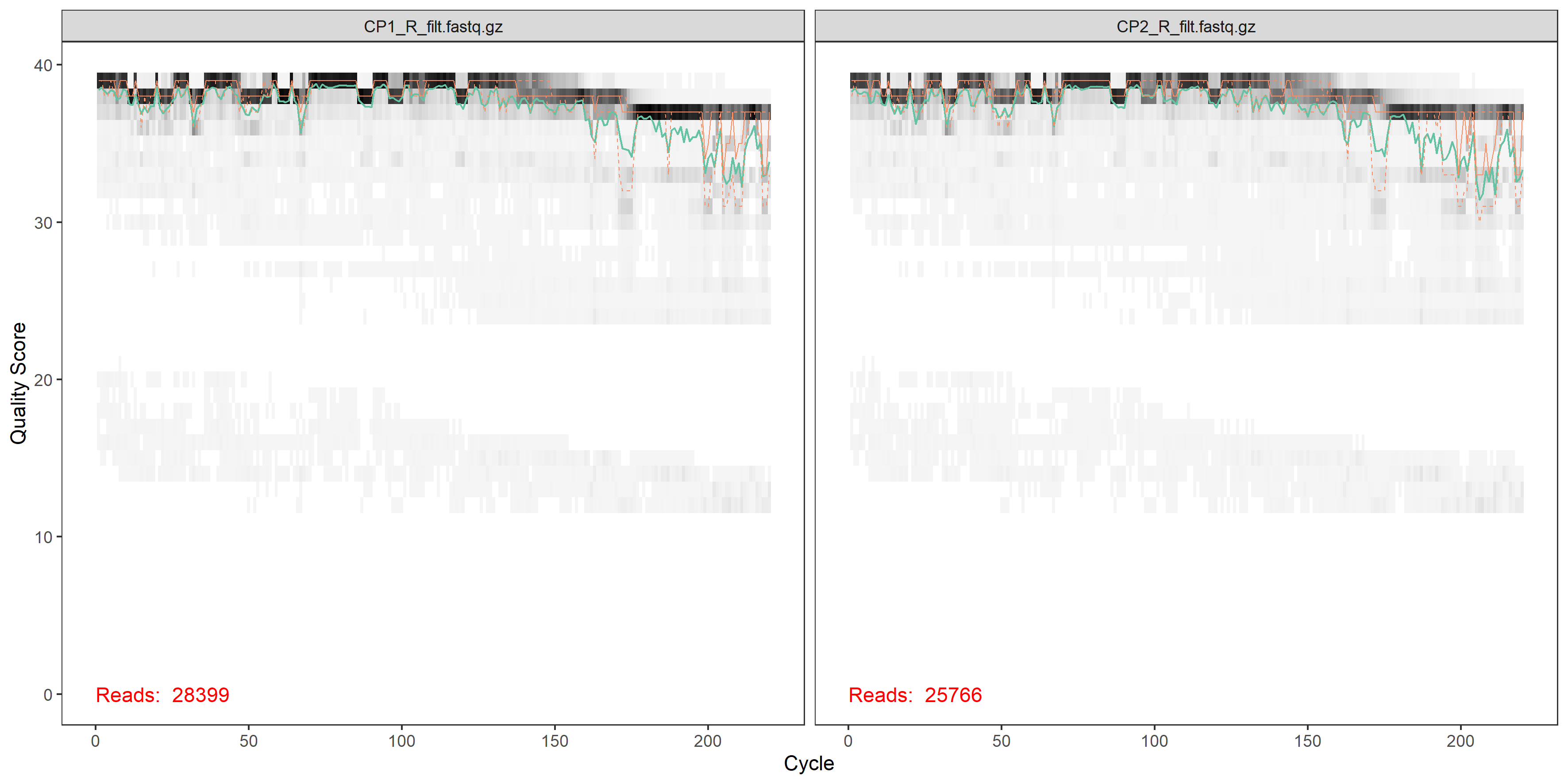
Assess and plot errors
errF <- learnErrors(filtFs, multithread=TRUE)
errR <- learnErrors(filtRs, multithread=TRUE)

plotErrors(errF, nominalQ=TRUE)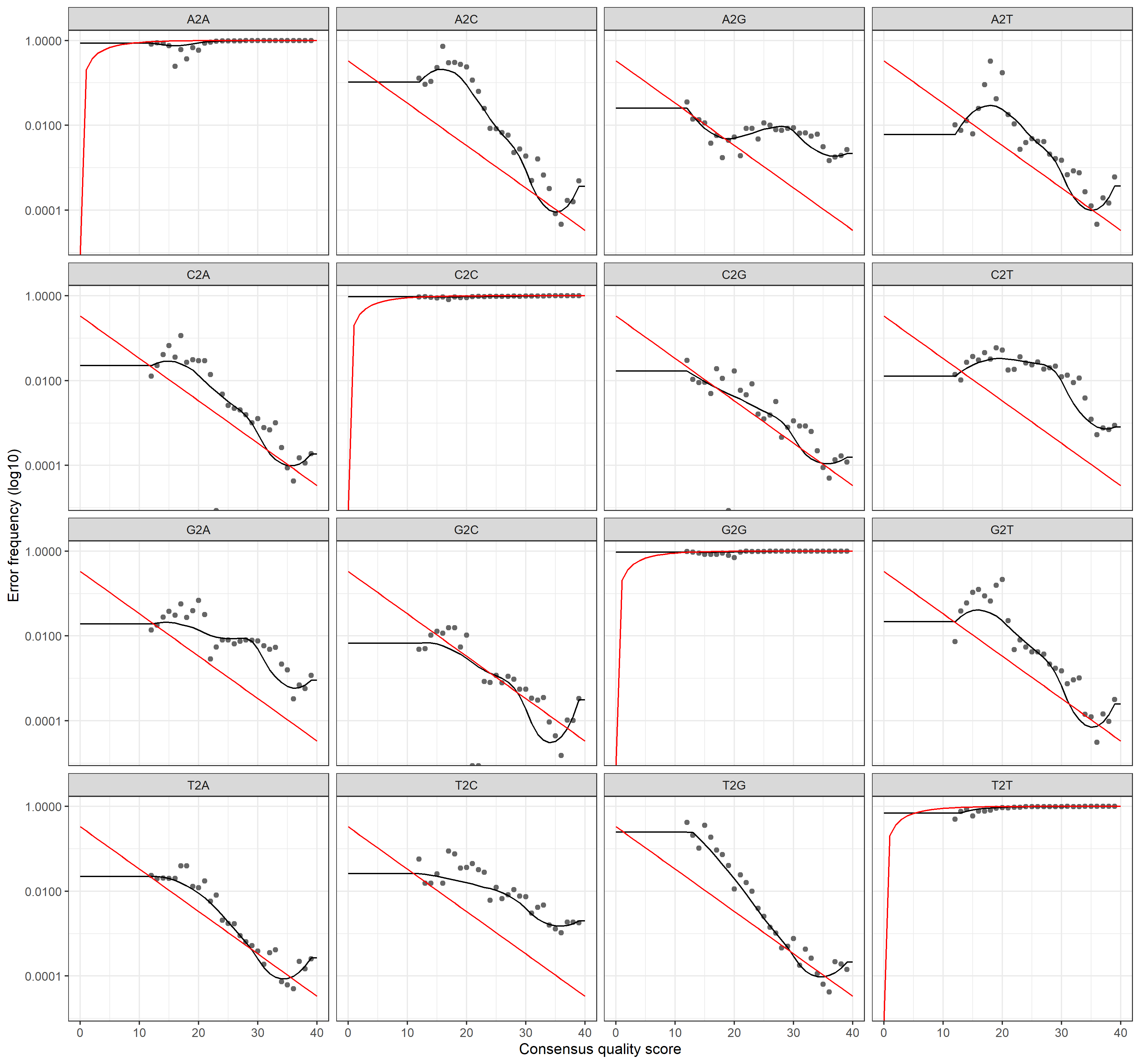
plotErrors(errR, nominalQ=TRUE)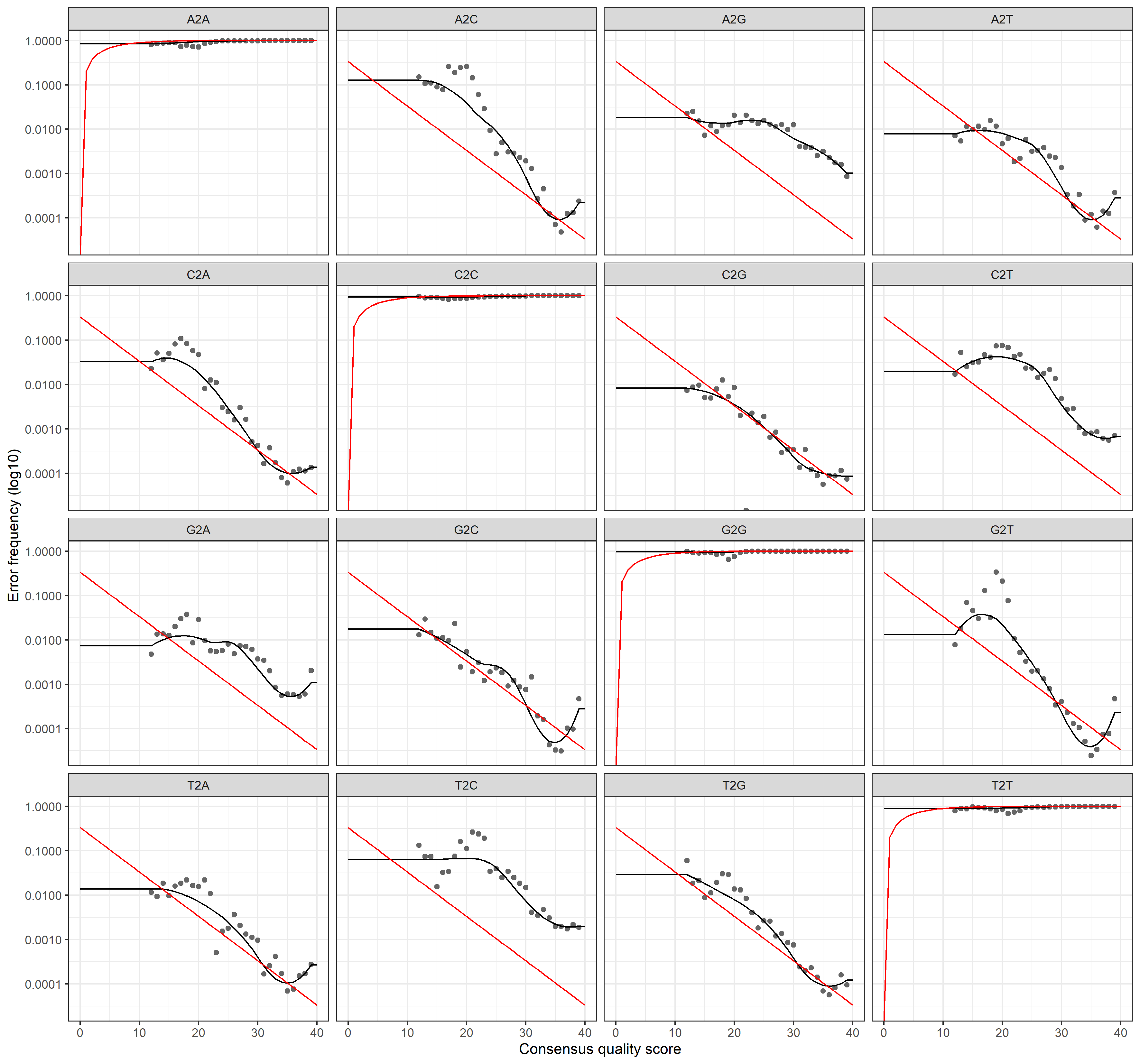
Dereplicate
derepFs <- derepFastq(filtFs, verbose=TRUE)
derepRs <- derepFastq(filtRs, verbose=TRUE)

# Name the derep-class objects by the sample names
names(derepFs) <- sample.names
names(derepRs) <- sample.names
Sample inference
dadaFs <- dada(derepFs, err=errF, multithread=TRUE)
dadaRs <- dada(derepRs, err=errR, multithread=TRUE)
Merge paired reads
mergers <- mergePairs(dadaFs, derepFs, dadaRs, derepRs, verbose=TRUE)Generate sequence table
seqtab <- makeSequenceTable(mergers)

# Inspect distribution of sequence lengths
table(nchar(getSequences(seqtab)))
Filter expected range
seqtab_subset <- seqtab[,nchar(colnames(seqtab)) %in% seq(426,428)]

# Inspect distribution of sequence lengths
table(nchar(getSequences(seqtab_subset)))
Remove chimeras
seqtab_subset.nochim <- removeBimeraDenovo(seqtab_subset,
                                           method="consensus",
                                           multithread=TRUE,
                                           verbose=TRUE)

dim(seqtab_subset.nochim)

sum(seqtab_subset.nochim)/sum(seqtab_subset)
Track reads through the pipeline
getN <- function(x) sum(getUniques(x))

track <- cbind(out,
               sapply(dadaFs, getN),
               sapply(dadaRs, getN),
               sapply(mergers, getN),
               rowSums(seqtab_subset.nochim))

colnames(track) <- c("input", "filtered", "denoisedF", "denoisedR", "merged", "nonchim")
rownames(track) <- sample.names

head(track)Assign taxonomy
taxa <- assignTaxonomy(seqtab_subset.nochim, "../silva_nr_v132_train_set.fa.gz", multithread=TRUE)

taxa.print <- taxa # Removing sequence rownames for display only
rownames(taxa.print) <- NULL
head(taxa.print)Export results
write.csv2(seqtab.nochim, "../output/16S-asvmat.csv", row.names = T)
write.csv2(taxa, "../output/16S-taxmat.csv", row.names = T)
Data preparation
Ordering and colors
# Default order for ID and Stage variables
order_id <- c('GS', 'GU', 'LH', 'CP', 'FA', 'WS', 'EA', 'EO', 'EC', 'ES')
order_stage <- c('Larva', 'Pupa', 'Adult', 'Eggs')

# Default color palettes for ID, Stage, and Label variables
cols_stage <- c('Larva' = '#C6AC8F', 'Pupa' = '#5E503F', 'Adult' = '#0A0908', 'Eggs' = '#EAE0D5')

cols_label <- c('Larval haemolymph' = '#C7928F', 'Larval gut unsterile' = '#A35752',
                'Larval gut sterile' = '#DDBDBB', 'Pupal cell pulp' = '#5E413F',
                'Female abdomen' = '#4F4740', 'Wash solution' = '#70655C',
                'Eggs cage' = '#F1E0D0', 'Eggs ovarium' = '#E3C1A1',
                'Eggs oviposition apparatus' = '#D09762', 'Eggs sterile' = '#C78243')

cols_id <- c('LH' = '#C7928F', 'GU' = '#A35752', 'GS' = '#DDBDBB', 'CP' = '#5E413F',
             'FA' = '#4F4740', 'WS' = '#70655C', 'EC' = '#F1E0D0', 'EO' = '#E3C1A1',
             'EA' = '#D09762', 'ES' = '#C78243')
Load the data
asvmat <- read.csv("../data/dada2-output/16S-asvmat.csv", sep = ";", row.names = 1)
taxmat <- read.csv("../data/dada2-output/16S-taxmat.csv", sep = ";", row.names = 1)
metmat <- read.csv("../data/metadata.csv", sep = ";")

# Compare and check sequences, assign ASV labels to replace sequences in tables
seq_check <- data.frame(ASV_SEQS = colnames(otumat),
                        TAX_SEQS = rownames(taxmat),
                        ASV = paste0('OTU', seq(1:nrow(taxmat)))) %>%
  mutate(TEST = ifelse(.$ASV_SEQS == .$TAX_SEQS, 1, 0))

# Sanity check to see if sequences in ASV and taxonomy table match
any(seq_check$TEST == 0) # If any values are 0, seqs do not match
Prepare tables
asvmat <- data.frame(t(asvmat)) %>%
  rownames_to_column('ASV_SEQS') %>%
  left_join(seq_check %>% select(ASV_SEQS, ASV)) %>%
  column_to_rownames('ASV') %>%
  select(-ASV_SEQS)

taxmat <- taxmat %>%
  rownames_to_column('TAX_SEQS') %>%
  left_join(seq_check %>% select(TAX_SEQS, ASV)) %>%
  column_to_rownames('ASV') %>%
  select(-TAX_SEQS)
Create phyloseq object
ps <- phyloseq(
  otu_table(as.matrix(asvmat), taxa_are_rows = T),
  tax_table(as.matrix(taxmat)),
  sample_data(metmat %>% column_to_rownames('SampleID')))
Explore the phyloseq object
sample_variables(ps) # check available metadata variables
sample_names(ps) # check sample names
sample_data(ps) # check metadata table

# Make sure the variables are plotted in the right order
sample_data(ps)$ID <- factor(sample_data(ps)$ID, levels = order_id)
sample_data(ps)$Stage <- factor(sample_data(ps)$Stage, levels = order_stage)
Rarefaction
rarecurve(t(otu_table(ps)), step=50, cex=0.5)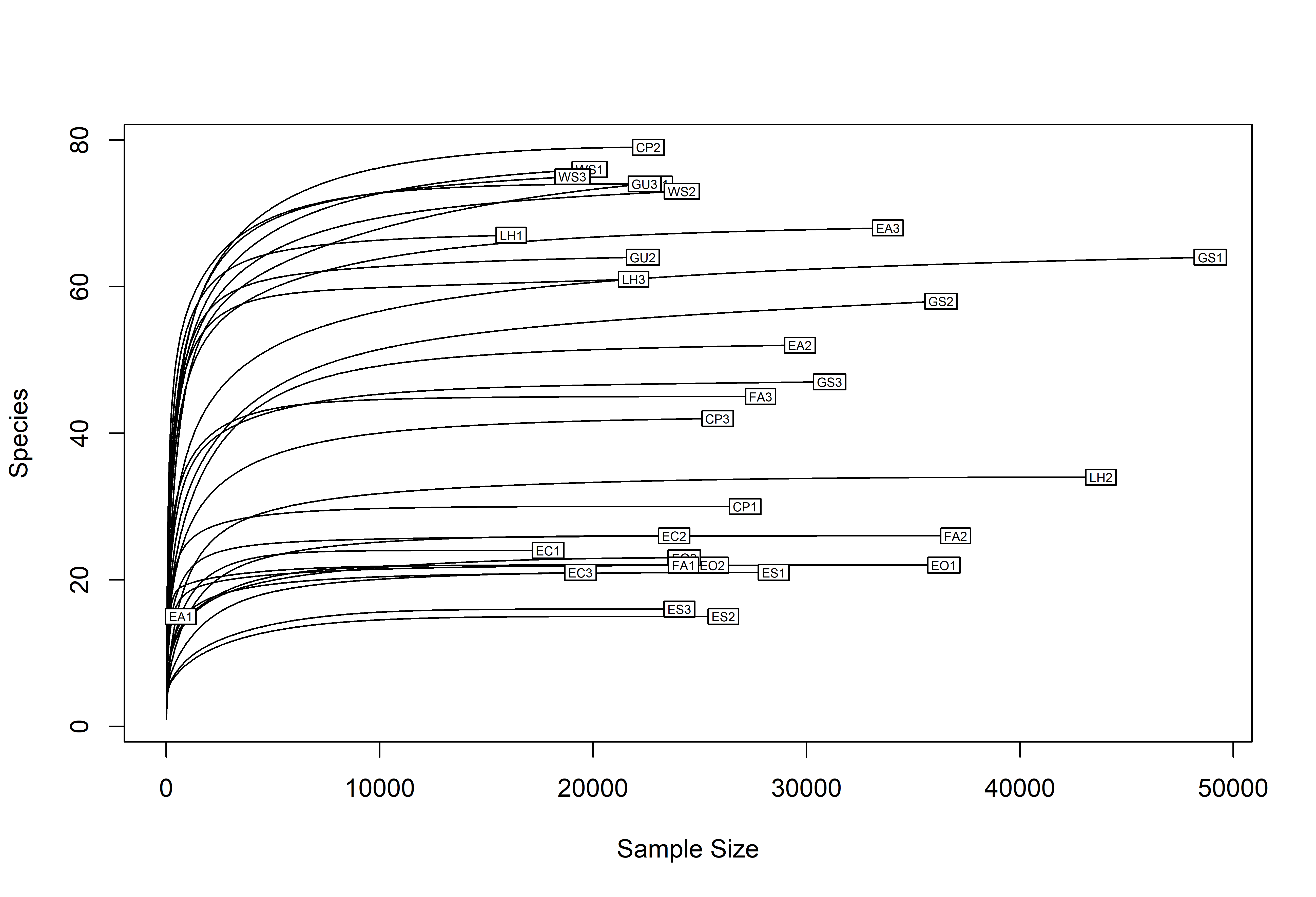
Remove outlier and rarefy
# Check smallest sample size
min(sample_sums(ps))

# Remove smallest sample
ps.sub <- subset_samples(ps, sample_names(ps) != 'EA1')

# Check again for smallest sample size and remaining number of samples
min(sample_sums(ps.sub))
nsamples(ps.sub)

# Rarefy abundance data to even depth and plot rarefaction curves
ps.rarefied <- rarefy_even_depth(ps.sub,
                                 rngseed = 1000,
                                 sample.size = min(sample_sums(ps.sub)),
                                 replace = F)

rarecurve(t(otu_table(ps.rarefied)), step=50, cex=0.5)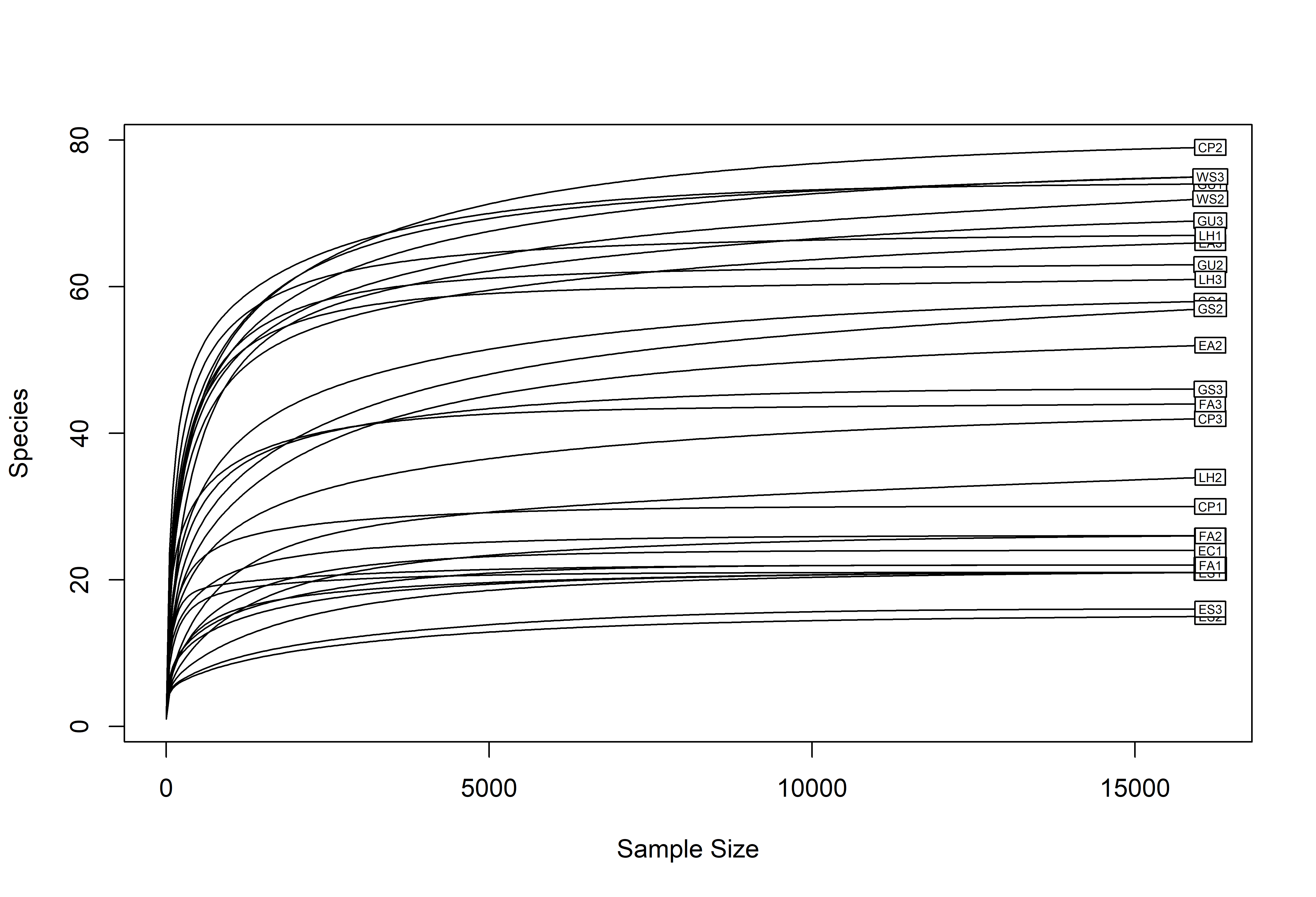
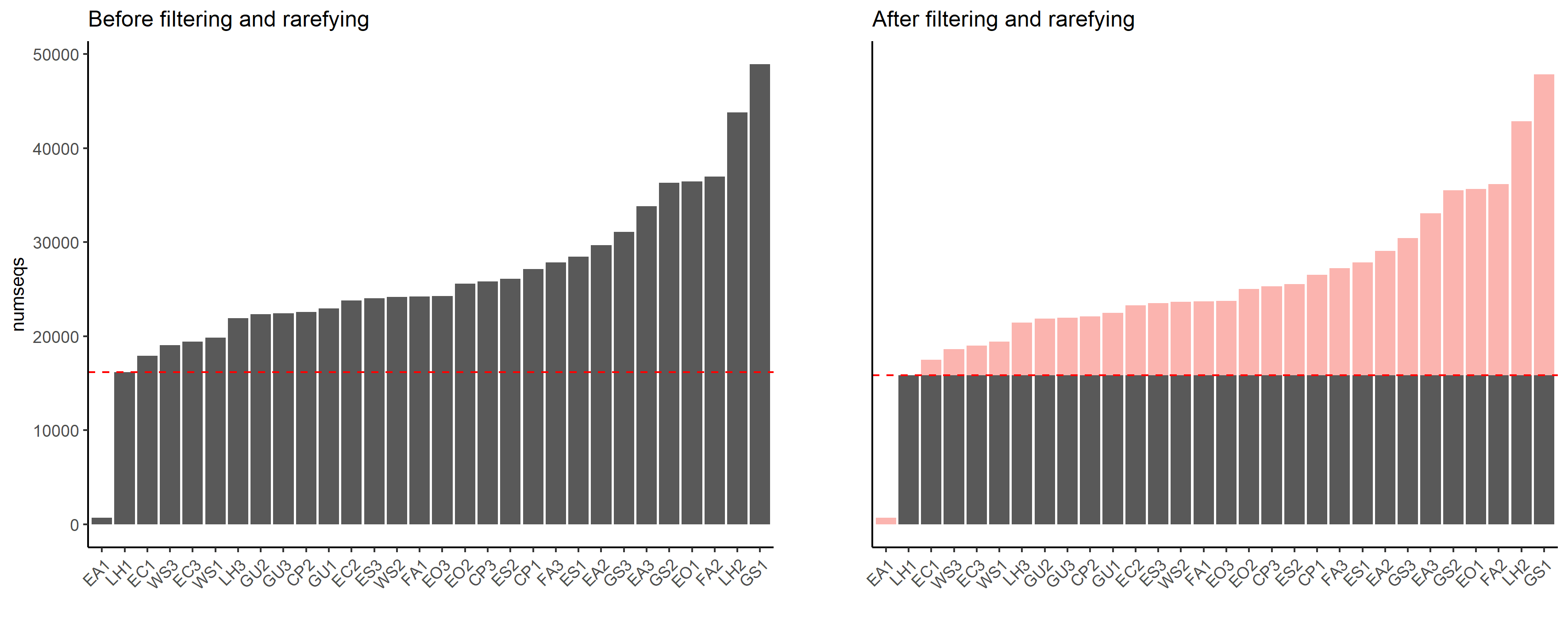
Before and after filtering and rarefying
Sample EA1 was removed from the dataset due to significantly lower read numbers. The remaining dataset was rarefied to the smallest sample size, thus, obtaining a dataset with equal sequencing depth.
Convert phyloseq object to ampvis2 object
amp.rarefied <- phyloseq_to_ampvis2(ps.rarefied)Credits to Kasper Skytte Anderson github.com/KasperSkytte for writing this function
This file contains bidirectional Unicode text that may be interpreted or compiled differently than what appears below. To review, open the file in an editor that reveals hidden Unicode characters.
Learn more about bidirectional Unicode characters
| phyloseq_to_ampvis2 <- function(physeq) { | |
| stop("The phyloseq_to_ampvis2 function is deprecated. amp_load() now supports loading a phyloseq object directly.", call. = FALSE) | |
| } |
Statistics & Visualization
General overview
p1 <- ggplot(bac) +
  geom_bar(aes(x = ID, y = Rel_Abundance/3, fill = Family), stat = 'identity', position = 'stack') +
  scale_fill_manual(values = colorRampPalette(brewer.pal(12, 'Set3'))(length(unique(bac$Family))))+
  labs(x = '', y = 'Relative abundance [%]') +
  facet_grid(.~Stage, scales = 'free_x', space = 'free') +
  guides(fill = guide_legend(ncol = 1, title = element_blank())) +
  theme_classic()

p2 <- bac_sub %>% filter(Family == 'Enterobacteriaceae') %>%
  ggplot() +
  geom_bar(aes(x = ID, y = Rel_Abundance/3, fill = Genus), stat = 'identity', position = 'stack') +
  scale_fill_manual(values = cut_colors[enterobacteriaceae], name = "Enterobacteriaceae") +
  labs(x = '', y = 'Relative abundance [%]') +
  facet_grid(.~Stage, scales = 'free_x', space = 'free_x') +
  theme_classic() +
  theme(legend.position = 'left')

p3 <- bac_sub %>% filter(Family == 'Burkholderiaceae') %>%
  ggplot() +
  geom_bar(aes(x = ID, y = Rel_Abundance/3, fill = Genus), stat = 'identity', position = 'stack') +
  scale_fill_manual(values = cut_colors[burkholderiaceae], name = "Burkholderiaceae") +
  lims(y = c(0, 100)) +
  facet_grid(.~Stage, scales = 'free_x', space = 'free_x') +
  theme_classic() +
  theme(legend.position = 'right')

ggarrange(
  p1 +
    theme(legend.position = 'bottom',
          legend.title = element_text(angle = 90),
          legend.margin = margin(-10, 0, 20, 0)) +
    guides(fill = guide_legend(nrow = 4, title.hjust = 0.5)),
  ggarrange(p2 +
              scale_y_continuous(breaks = c(0, 25, 75, 100), position = 'right', limits = c(0, 100)) +
              theme(axis.text.y.right = element_text(hjust = 0.5, vjust = 6, angle = 270),
                    axis.title.y.right = element_text(size = 9)) +
              guides(fill = guide_legend(label.position = 'left', label.hjust = 1)),
            p3 +
              theme(axis.text.y = element_blank(),
                    axis.title.y = element_blank()),
            labels = c('B', 'C'), label.y = 1.05, font.label = list(color = 'grey45', face = 'bold')),
  nrow = 2, heights = c(1.1, 0.8), labels = c('A'),font.label = list(color = 'grey45', face = 'bold'))
# Rarefy all samples
ps.rarefied.full <- rarefy_even_depth(ps,
sample.size = min(sample_sums(ps)),
rngseed = 1000,
replace = F)
# Construct table containing abundance, taxonomy, and meta information
bac <- data.frame(t(otu_table(ps.rarefied.full))) %>%
rownames_to_column('SampleID') %>%
melt(variable.name = 'ASV', value.name = 'Abundance') %>%
left_join(data.frame(tax_table(ps.rarefied.full)) %>%
rownames_to_column('ASV')) %>%
filter(!is.na(Family)) %>%
group_by(SampleID) %>%
mutate(Rel_Abundance = Abundance/sum(Abundance)*100) %>%
left_join(data.frame(sample_data(ps.rarefied.full)) %>%
rownames_to_column('SampleID') %>%
select(SampleID, ID, Stage, Label)) %>%
mutate(ID = factor(ID, levels = order_id),
Stage = factor(Stage, levels = c('Larva', 'Pupa', 'Adult', 'Eggs')))
# Subset families of Burkholderiaceae and Enterobacteriaceae
bac_sub <- bac %>%
filter(Family %in% c('Burkholderiaceae', 'Enterobacteriaceae')) %>%
mutate(Genus = gsub("-", "-\n ", Genus))
cut_colors <- setNames(colorRampPalette(brewer.pal(12, 'Set3'))(length(unique(bac_sub$Genus))), levels(factor(bac_sub$Genus)))
burkholderiaceae <- bac_sub %>% filter(Family == 'Burkholderiaceae') %>% .$Genus %>% unique()
enterobacteriaceae <- bac_sub %>% filter(Family == 'Enterobacteriaceae') %>% .$Genus %>% unique()
click figure to see larger version
Alpha diversity
Create comprehensive alpha diversity table
alpha <- alpha(ps.rarefied, index = 'all')Prepare data for plotting
# Extract metadata
ps.rarefied.meta <- meta(ps.rarefied)

# Add selected alpha diversity measures to metadata table
ps.rarefied.meta$Shannon <- alpha$diversity_shannon
ps.rarefied.meta$Evenness <- alpha$evenness_pielou

# Set order and grouping for statistics
levels_stage <- levels(as.factor(ps.rarefied.meta$Stage))
pairs_stage <- combn(seq_along(levels_stage), 2, simplify = F, FUN = function(i)levels_stage[i])
Plot alpha diversity measures and add statics
# Set shapes for each group of samples
shapes_id <- c('LH' = 16, 'GU' = 17, 'GS' = 18, 'CP' = 16, 'FA' = 16, 'WS' = 17, 'EC' = 16, 'EO' = 17, 'EA' = 18, 'ES' = 15)

# Plot alpha diversity values
shannon_p <- ggplot(ps.rarefied.meta, aes(x = Stage, y = Shannon)) +
  geom_violin(aes(fill = Stage),
              colour = NA, trim = F, alpha = 0.4) +
  geom_point(aes(colour = ID, shape = ID),
             size = 4, position = position_jitter(width = 0.15, seed = 12)) +
  geom_boxplot(aes(fill = Stage),
               colour = 'white', width = 0.2, alpha = 0.25) +
  scale_fill_manual(values = cols_stage) +
  scale_color_manual(values = cols_id) +
  scale_shape_manual(values = shapes_id) +
  labs(x = 'Developmental stage',
       y = 'Shannon index',
       colour = '',
       shape = '') +
  guides(fill = 'none') +
  theme_classic()

# Add statistics
shannon_p <- shannon_p + stat_compare_means(aes(label = ..p.signif..), comparisons = pairs_stage, ref.group = '0.5', method = 'wilcox.test')

# Assign sample groups to developmental stages to subset legend
larva <- c('LH', 'GU', 'GS')
pupa <- c('CP')
adult <- c('FA', 'WS')
eggs <- c('EC', 'EO', 'EA', 'ES')

# Create separate legends for each developmental stage
legend_larva <- get_legend(
  ggplot(ps.rarefied.meta %>% filter(Stage == 'Larva'),
         aes(x = Stage, y = Shannon)) +
    geom_point(aes(colour = ID, shape = ID),
               size = 4, position = position_jitter(width = 0.15, seed = 12)) +
    labs(fill = 'Larva', colour = 'Larva', shape = 'Larva') +
    scale_fill_manual(values = cols_stage[larva]) +
    scale_color_manual(values = cols_id[larva]) +
    scale_shape_manual(values = shapes_id[larva]))

legend_pupa <- get_legend(
  ggplot(ps.rarefied.meta %>% filter(Stage == 'pupa'),
         aes(x = Stage, y = Shannon)) +
    geom_point(aes(colour = ID, shape = ID),
               size = 4, position = position_jitter(width = 0.15, seed = 12)) +
    labs(fill = 'Pupa', colour = 'Pupa', shape = 'Pupa') +
    scale_fill_manual(values = cols_stage[pupa]) +
    scale_color_manual(values = cols_id[pupa]) +
    scale_shape_manual(values = shapes_id[pupa]))

legend_adult <- get_legend(
  ggplot(ps.rarefied.meta %>% filter(Stage == 'adult'),
         aes(x = Stage, y = Shannon)) +
    geom_point(aes(colour = ID, shape = ID),
               size = 4, position = position_jitter(width = 0.15, seed = 12)) +
    labs(fill = 'Adult', colour = 'Adult', shape = 'Adult') +
    scale_fill_manual(values = cols_stage[adult]) +
    scale_color_manual(values = cols_id[adult]) +
    scale_shape_manual(values = shapes_id[adult]))

legend_eggs <- get_legend(
  ggplot(ps.rarefied.meta %>% filter(Stage == 'eggs'),
         aes(x = Stage, y = Shannon)) +
    geom_point(aes(colour = ID, shape = ID),
               size = 4, position = position_jitter(width = 0.15, seed = 12)) +
    labs(fill = 'Eggs', colour = 'Eggs', shape = 'Eggs') +
    scale_fill_manual(values = cols_stage[eggs]) +
    scale_color_manual(values = cols_id[eggs]) +
    scale_shape_manual(values = shapes_id[eggs]))

# Arrange legends
legends <- ggarrange(legend_larva, legend_pupa, legend_adult, legend_eggs, nrow = 4, heights = c(0.4, 0.2, 0.3, 0.5))

# Combine the alpha diversity plot with its legends
shannon_p <- ggarrange(shannon_p + theme(legend.position = 'none'), ggarrange(legends,nrow = 2, heights = c(0.6, 0.4)), ncol = 2, widths = c(1.8, 0.3))

shannon_p
click figure to see larger version
pielou_p <- ggplot(ps.rarefied.meta, aes(x = Stage, y = Evenness)) +
  geom_violin(aes(fill = Stage), colour = NA, trim = F, alpha = 0.4) +
  geom_point(aes(colour = ID, shape = Tissue), size = 4, position = position_jitter(width = 0.15, seed = 12)) +
  geom_boxplot(aes(fill = Stage), colour = 'white', width = 0.2, alpha = 0.25) +
  scale_fill_manual(values = cols_stage) +
  scale_color_manual(values = cols_id) +
  labs(x = 'Developmental stage',
       y = 'Shannon index',
       colour = '',
       shape = '') +
  guides(fill = 'none') +
  theme_classic()

pielou_p <- pielou_p + stat_compare_means(aes(label = ..p.signif..), comparisons = pairs_stage, ref.group = '0.5', method = 'wilcox.test')

pielou_p
click figure to see larger version
amp_rankabundance(amp.rarefied, group_by = 'Stage', showSD = TRUE, log10_x = TRUE) +
  scale_colour_manual(values = cols_stage) +
  scale_fill_manual(values = cols_stage)
click figure to see larger version
Venn diagrams
# Group samples based on developmental stage

venn_p1 <- ps_venn(ps.rarefied,
                   group = 'Stage',
                   fill = cols_stage,
                   colour = 'white',
                   edges = F,
                   alpha = 0.5)
venn_p1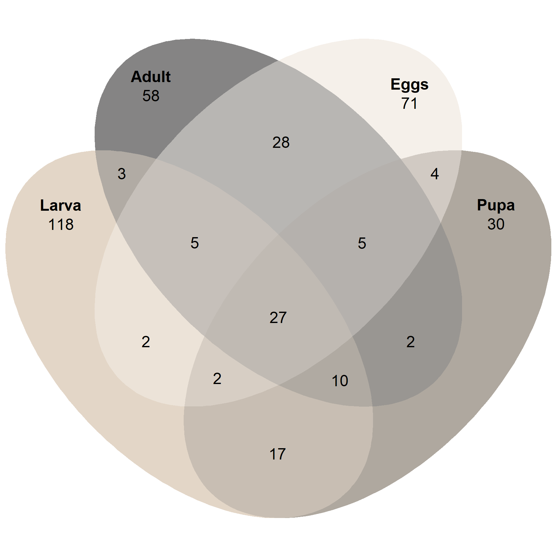
ps_egg <- subset_samples(ps.rarefied, Stage == 'Eggs')

venn_p2 <- ps_venn(ps_egg,
                   group = 'ID',
                   fill = c('EA' = '#D09762', 'EO' = '#E3C1A1', 'EC' = '#F1E0D0', 'ES' = '#C78243'),
                   colour = 'white',
                   edges = F,
                   alpha = 0.5)
venn_p2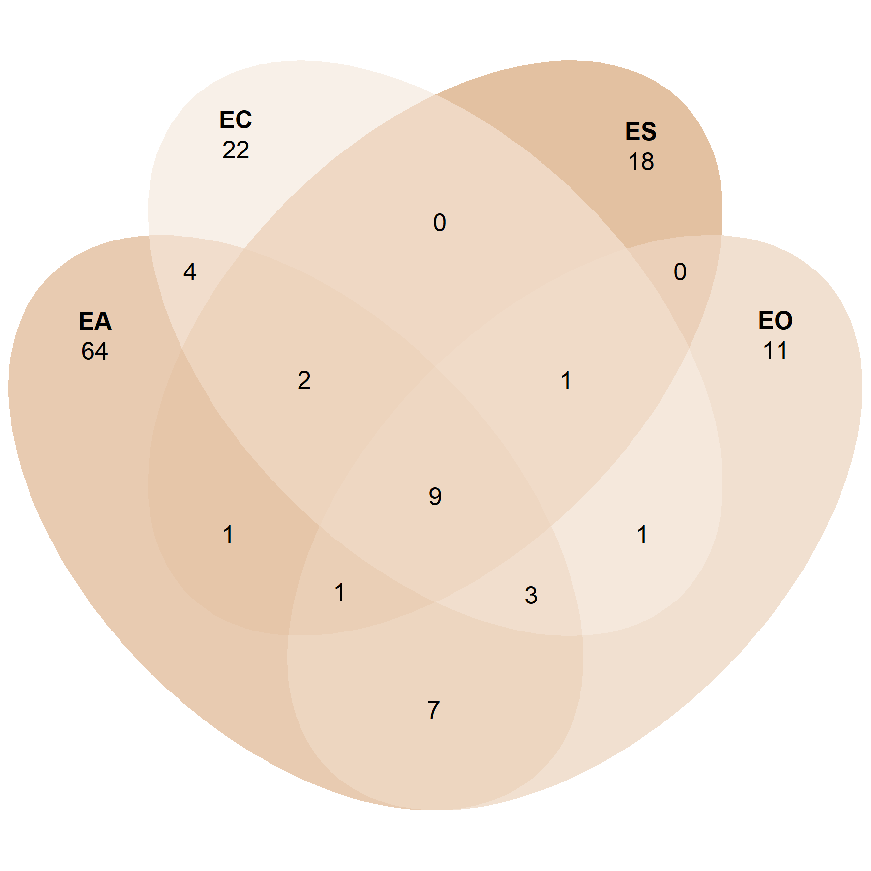
ps_lar <- subset_samples(ps.rarefied, Stage == 'Larva')

venn_p3 <- ps_venn(ps_lar,
                   group = 'ID',
                   fill = c('GS' = '#DDBDBB', 'GU' = '#A35752', 'LH' = '#C7928F'),
                   colour = 'white',
                   edges = F,
                   alpha = 0.5)
venn_p3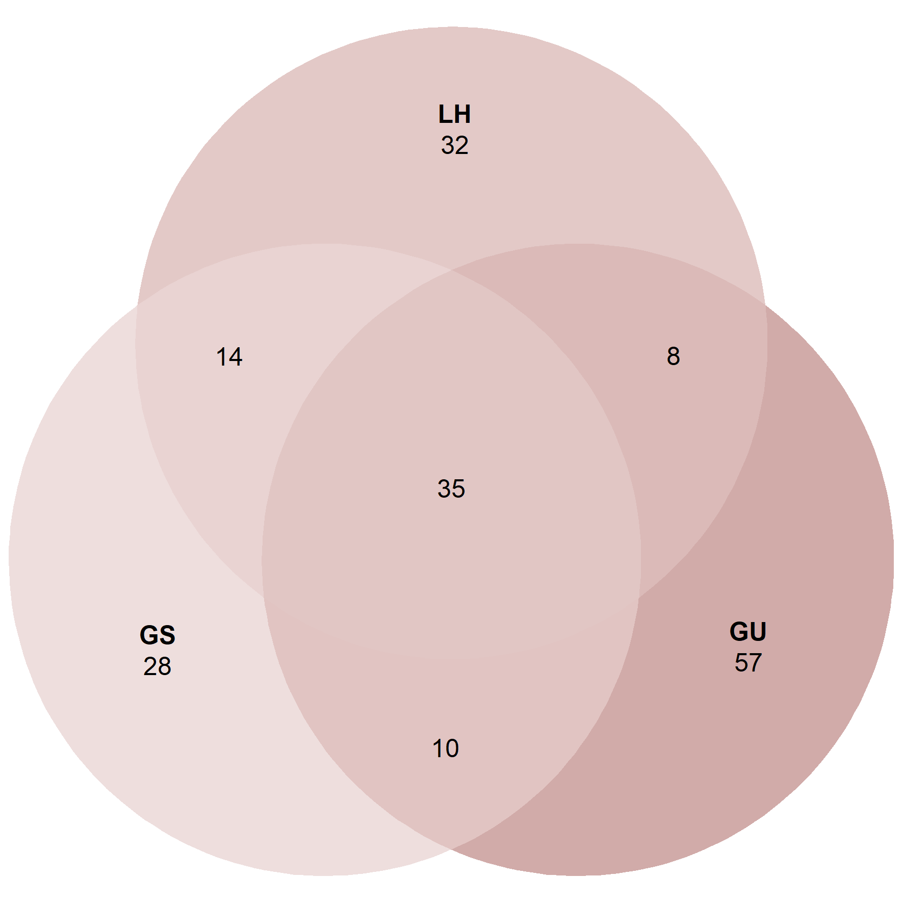
ps_adu <- subset_samples(ps.rarefied, Stage == 'Adult')

venn_p4 <- ps_venn(ps_adu,
                   group = 'ID',
                   fill = c('FA' = '#4F4740', 'WS' = '#70655C'),
                   colour = 'white',
                   edges = F,
                   alpha = 0.5)
venn_p4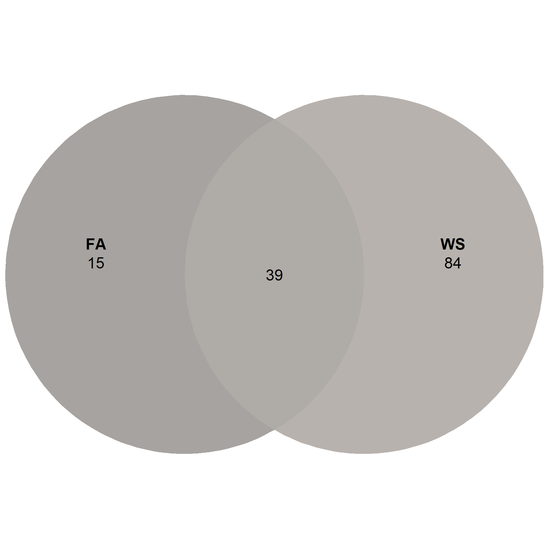
ps_adu_egg <- subset_samples(ps.rarefied, ID %in% c('FA', 'WS', 'EA', 'EO'))

venn_p5 <- ps_venn(ps_adu_egg,
                   group = 'ID',
                   fill = c('FA' = '#4F4740', 'WS' = '#70655C', 'EA' = '#D09762', 'EO' = '#E3C1A1'),
                   colour = 'white',
                   edges = F,
                   alpha = 0.5)
venn_p5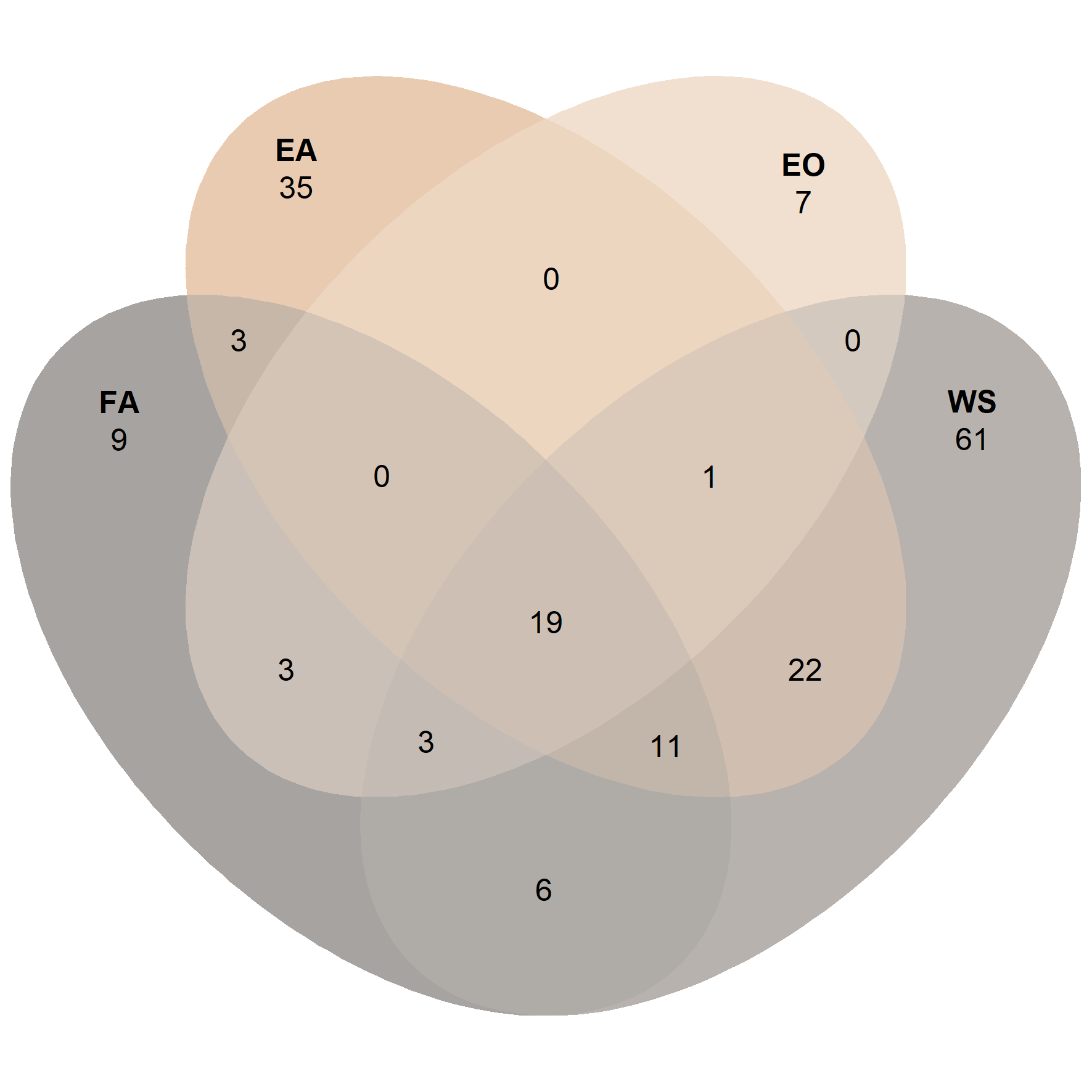

click figure to see larger version
Heatmap
Plot heatmap
amp_heatmap(
  amp.rarefied,
  group_by = 'SampleID',
  facet_by = 'Stage',
  tax_aggregate = 'Genus',
  tax_add = 'Phylum',
  tax_show = 25,
  normalise = T,
  showRemainingTaxa = T,
  plot_values_size = 3,
  color_vector = c('white', '#A2708A'),
  plot_colorscale = 'sqrt',
  plot_values = F) +
  theme(axis.text.x = element_text(angle = 45, size = 8, vjust = 1),
        axis.text.y = element_text(size = 8),
        legend.position='right')
click figure to see larger version
Ordination
Canonical Correspondence Analysis
ordinationresult <- amp_ordinate(
  amp.rarefied,
  type = 'CCA',
  constrain = 'ID',
  transform = 'Hellinger',
  sample_color_by = 'Stage',
  sample_colorframe = TRUE,
  sample_colorframe_label_size = 4,
  sample_colorframe_label = 'Stage',
  sample_label_by = 'ID',
  sample_label_size = 3.5,
  repel_labels = T,
detailed_output = T)ordinationresult$plot +
scale_fill_manual(values = cols_stage) +
scale_colour_manual(values = cols_stage) +
labs(fill = '', colour = '') +
theme_classic() +
theme(legend.position = 'none')
click figure to see larger version
ordinationresult$screeplot
click figure to see larger version
Permanova
# Prepare data
abund_tab <- data.frame(t(otu_table(ps.rarefied)))
group_tab <- data.frame(sample_data(ps.rarefied)) %>% rownames_to_column('SampleID')set.seed(123)
adonis_stage <- adonis(abund_tab ~ Stage, data = group_tab, permutations = 1000, method = 'bray')
adonis_stage## Permutation: free
## Number of permutations: 1000
##
## Terms added sequentially (first to last)
##
## Df SumsOfSqs MeanSqs F.Model R2 Pr(>F)
## Stage 3 3.9545 1.31815 12.676 0.60335 0.000999 ***
## Residuals 25 2.5997 0.10399 0.39665
## Total 28 6.5541 1.00000
## ---
## Signif. codes: 0 '***' 0.001 '**' 0.01 '*' 0.05 '.' 0.1 ' ' 1set.seed(123)
adonis_tissue <- adonis(abund_tab ~ Tissue, data = group_tab, permutations = 1000, method = 'bray')
adonis_tissue## Permutation: free
## Number of permutations: 1000
##
## Terms added sequentially (first to last)
##
## Df SumsOfSqs MeanSqs F.Model R2 Pr(>F)
## Tissue 4 3.6108 0.90270 7.3607 0.55092 0.000999 ***
## Residuals 24 2.9433 0.12264 0.44908
## Total 28 6.5541 1.00000
## ---
## Signif. codes: 0 '***' 0.001 '**' 0.01 '*' 0.05 '.' 0.1 ' ' 1Pairwise Permanova
set.seed(123)
ppermanova_stage <- pairwise.perm.manova(vegdist(abund_tab, method = 'bray'), group_tab$Stage, nperm = 1000, p.method = 'bonferroni')
ppermanova_stage
##
## Pairwise comparisons using permutation MANOVAs on a distance matrix
##
## data: vegdist(abund_tab, method = "bray") by group_tab$Stage
## 1000 permutations
##
## Larva Pupa Adult
## Pupa 0.042 - -
## Adult 0.012 0.156 -
## Eggs 0.006 0.048 0.006
##
## P value adjustment method: bonferroniset.seed(123)
ppermanova_tissue <- pairwise.perm.manova(vegdist(abund_tab, method = 'bray'), grouping$Tissue, nperm = 1000, p.method = 'bonferroni')
ppermanova_tissue##
## Pairwise comparisons using permutation MANOVAs on a distance matrix
##
## data: vegdist(abund_tab, method = "bray") by grouping$Tissue
## 1000 permutations
##
## Eggs Gut Haemolymph Ovarium
## Gut 0.02 - - -
## Haemolymph 0.01 0.04 - -
## Ovarium 0.16 0.15 0.52 -
## Ovipositor 0.06 0.03 1.00 0.87
##
## P value adjustment method: bonferroniLefSe
lefse <- run_lefse(ps.rarefied,
                   group = 'Stage',
                   taxa_rank = 'Genus')
Plot
plot_ef_bar(x) +
  scale_fill_manual(values = cols_stage) +
  theme_classic() +
  theme(legend.title = element_blank(),
        legend.position = c(0.8, 0.1))
click figure to see larger version
Network
library(ggrepel)

set.seed(100)

ig <- make_network(ps.rarefied, max.dist = 0.5, distance = 'bray')

plot_network(ig, ps.rarefied, color = 'Stage', point_size = 4, type = 'samples', label = NA) +
  geom_text_repel(aes(label = value), size = 3.5, box.padding = 0.5) +
  scale_colour_manual(values = cols_stage) +
  theme(legend.position = c(0.8, 0.2))
click figure to see larger version